Open Access
Review Article
Max Screen >>
ISSN: 2455-765X
Copyright: © 2015 Bianciardi G. This is an open-access article distributed under the terms of the Creative Commons Attribution License, which permits unrestricted use, distribution, and reproduction in any medium, provided the original author and source are credited.
Related article at Pubmed, Google Scholar
Fractal analysis is an objective and sensitive approach that has become very useful in the understanding of many phenomena in various fields. In pathology we have one of the most important fields of application. Here we review and present fractal methodologies that have been successfully applied by us in order to characterize pathological features and perform differential diagnosis of cancer and atherosclerosis-linked diseases, the most common diseases of the present day. Congenital disorder characterization can be equally benefit by the use of these morphometric approaches.
Keywords: Fractal geometry; Pathology; Fractal analysis
Mandelbrot’s concept of fractal geometry has improved our ability to characterize natural structures and shapes, bringing essential contributions to the comprehension of complex systems and chaos in nature.
The term “fractal” as associated to a curve, a surface or any other geometrical domain, that subtends the mathematical property of having fractional dimensions. This new concept characterizes the fractal geometry and distinguishes it from the traditional Euclidean geometry, in which any objects must have integer dimension. Mandelbrot showed that a suitable method to define a fractal curve (or surface) is to adopt the concept of “self-similarity”. In theoretical fractal a self-similar structure has the same appearance and the same geometric properties when examined at any level of magnification (or scales). In this sense this structure is said to be self-similar. A fractal curve (e.g. self-similar) can have a not null area because the length of the curve branch bounded by a surface domain of finite area can be infinite. Unlike a smooth line, a fractal curve, which has a dimension between 1 and 2, can be irregular or wrinkly.
Over 100 years ago first-rate mathematicians such as Georg Cantor and Giuseppe Peano had already produced results that seemed to supersede concepts that had been taken for granted such as the concept of dimension, area and perimeter. The first attack on the common way of looking at these concepts took place in the second half of the nineteenth century. On 20th June 1877, a young Georg Cantor, yet to become professor at the University of Halle, wrote a letter to his German friend and senior colleague J.W.R Dedekind. In tiny, neat handwriting, Cantor wrote that he was in possession of results proving that a square owns a number of points no higher than the number of each of its sides. Dimension of 1 and dimension of 2 are the same? How could the concept of dimension be saved? For their part, the Italian G. Peano and the Pole W. Sierpiński had begun to produce strange mathematical entities which were infinitely irregular and capable of repeating the same for indefinitely. These Figures began to proliferate in their writings and in those of other mathematicians: in Helge von Koch curve (Figure 1) triangles could be seen breaking up into ever smaller triangles or, from a different point of view, triangles were born infinite times from the sides of other triangles. The perimeter of these Figures was infinite, while their areas were certainly finite and measurable.
Most mathematicians considered these strange forms a “museum of horrors”, a collection of “monsters” that could have no any equivalent in the real world. However, studies of these infinitely irregular figures continued for several years and their properties were emphasized: changing scale they are able to repeat themselves infinitely, they are characterized by self-similarity, or internal homothety. The last studies date back to the second decade of the twentieth century, in works by French mathematicians Pierre Fatou and Gaston Julia. Subsequently, nothing was heard of these “mathematical monsters” for many years. What physical significance could curves with an infinite perimeter and finite area ever have?
Benoit B. Mandelbrot was born in Warsaw in 1924, to a Lithuanian Jewish family. When Mandelbrot was 12, his family moved to Paris, partly because of the atmosphere of racism that had begun to be felt in Europe. The fact that Benoit’s uncle was already in Paris, working as a professor of mathematics at the Collège de France, also influenced their move. The presence of the uncle was certainly a determining factor in the development of Benoit’s interest in mathematics. At the end of the war, Benoit enrolled at the École normale supérieure in Paris to study mathematics. His presence at the prestigious school lasted a matter of days, however. At that time the school of thought of a group of mathematicians who adopted the invented name of “Nicolas Bourbaki” prevailed in Paris. According to this group, all essential maths should be rewritten, based exclusively on logical criteria. They allowed no space for geometry, not the application of maths to real physical phenomena. Mandelbrot described that period as nightmarish: for him maths was geometry, the study of forms, and a powerful instrument for analysis of the physical world. He therefore enrolled at the Paris Polytechnic, where he met the elderly Julia, who spoke to him of his strange mathematical models. Mandelbrot was entranced.
To develop the heliocentric model, Galileo used a newly developed technical instrument: a telescope. Mandelbrot also used a newly technical instrument to develop his mathematical models and his vision of the world: the computer. In the 1950’s Mandelbrot left France to work at the IBM’s Thomas J. Watson Research Center in Yorktown Heights, New York, where he found the ideal tool for his studies. The study of noise on telephone lines soon lead him into the world of infinitely irregular and homothetic mathematical models. Mandelbrot realised that regularities could be seen between the periods without errors and the periods with errors: independently of whether the interval of time was considered, a second, a minute or an hour. Even when the time-scale changed, the relationship remained constant. For Mandelbrot’s geometric mind this represented the occurrence in nature of one of the “monsters” of the nineteenth century: the Cantor dust [1]. Mandelbrot was creating a new geometry. Classical geometry is based on lines and surfaces, circles and spheres, triangles and parallelepipeds: an abstraction of reality, based on (and the basis of) the Plato-Pythagoras tradition. So abstract, that it is wrong when applied to complexity. And the world is complexity. “Clouds are not spheres and mountains are not cones” – Mandelbrot would say- and irregularity is not an accident that distorts regular geometric forms, but rather the essence of the natural things. A bolt of lightning does not travel in a straight line, but in a complex, branching, irregular line. This is not the distortion of a hypothetical straight lines because, if one considers the distribution of zigzags, one realises that there is a completely new regularity within this complexity: the order of (statistical) self-similarity, or homothety. The birth of fractal geometry dates back to the publication of his paper “How long is the coast of Britain? Statistical self-similarity and fractal dimension” [2]. In this article, Mandelbrot maintained that a coastline has a perimeter that tends towards the infinite, although the area enclosed is certainly finite. Coastlines are self-similar: when the scale changes (e.g. with even more detailed and close-up photographs of the coast) the degree of irregularity of the coast remains essentially the same. The degree of irregularity could now be measured using the Hausdorff-Besicovitch concept of dimension in 1919, not as a mathematical curiosity, but as a powerful means of analysing the form of objects in nature. Thus, according that Mandelbrot paper, the concept of fractal dimension was born: the quantification of the probability that a given area is occupied by a fractal structure. A fractal line, such a coastline, has a fractional dimension between one and two (and a fractal surface, such as a mountain, has a dimension between two and three. A coastline is therefore nothing more than the realisation in nature of the Koch snowflake (and the name “fractal” having coined by Mandelbrot while flicking his nephew’s Latin dictionary: “fractus”, an irregular structure).
In effect, natural structures having fractal appearance have been found in a variety of natural and biological entities [3-9]: river deltas, trees, cardiopulmonary structures, the ramifying tracheo-bronchial tree, the His-Purkinje network, as well as the cardiac muscle bundles and the placenta’s arterial tree [10,11]. In biology, complex structures have no characteristic length: often they have fractal – or, more generally, scaling – properties. The meaning of these fractal structures in the human body is profound. The selfsimilar tracheo-bronchial tree provides an enormous surface area for exchange of gases at the vascular-alveolar interface, coupling pulmonary and cardiac functions, and fractal branching provides a rich network for distribution of nutrients and oxygen, as well for the collection of metabolic waste products [12,13]. Fractal structure serves function, e.g., the fractal organization of connective tissue in the aortic leaflets relating to the efficient distribution of mechanical forces [14]. They can be quantified by index like as the “fractal dimension”, D, measure of geometric complexity and of the space-filling properties of a structure [15], identified by Mandelbrot. Soon after, fractal analysis burst into pathology, differential diagnosis, prognosis and treatment of the patient.
To improve the effectiveness and safety of patient care, today there is a growing emphasis on differential diagnosis tools, in order to apply the best therapy to the patient. Also in the present “molecular days”, imaging is the actual cornerstone: radiodiagnostics by X-rays or radiochemical tracers, magnetic resonance imaging, positron-emission tomography (a functional imaging technique, particularly useful to explore the presence of cancer metastasis), and all techniques that are in the pathology lab: microscopies such as light microscopy, performed on biopsy and cytology specimens (by the routine hematoxylin-eosin staining, special stainings, and antibody stainings), as well transmission electron microscopy. Morphometry, the measure of shapes, can be added to every imaging technique in order to obtain objective indexes. In this field, since many years, fractal geometry has been applied to histopathology, cytopathology, and other biomedical domains with great success [16-19].
Performing fractal analysis of tissue samples, it’s possible to make differential diagnosis between the early stage of tumors and flogosis [20] or among the different types of Basal Cell Cancer, as well as to investigate the subtle alterations of the nuclear patterns in human breast tumors [21] or evaluate brain tumors [22]. Fractal analysis shows a high ability for automatic classification of cancer cells in urinary smears [23] as well as to identify prostate cancer cells [24]. Fractal analysis is able to provide quantitative information on the link among molecular, cellular and histomorphological tissue changes in the development of tumors [8,9].
The use of fractal analysis to analyze histological specimen, e.g to help in tumor diagnosis, may starts with the image analysis of the single-pixel specimen outlines in order to perform the evaluation of the geometric complexity or entropy present in the images. It may be performed by following the nuclei distribution in the tissue in order to perform a mass dimension technique [25], or by using the box-counting technique over the tissue outlines, as below described.
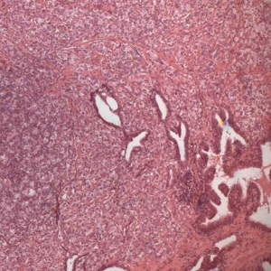
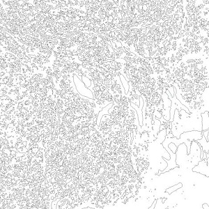
To perform computerized image analysis and to obtain morphometric fractal indices, the first challenge is the tissue/cell/nucleus segmentation, to separate noise and biological features. The second step is the feature selection to isolate the tissue, the cells, or the nuclei of interest. The last important challenge is the system of evaluation, e.g. the log-log plot in order to determine the fractal dimension of the skeletonized tissue/cell/nucleus, being the fractal dimension(s) the exponent of a log-log plot, meaning the self-similarity of the biological structure [26]. In a possible approach, images are digitized, aperture settings and conditions of illumination and magnification are kept constant. Single pixel outlines of the contours of the image are automatically obtained by using grey-level threshold segmentation (Figures 2 and 3; bottom, left) then fractal indexes are applied, making use of a computerized system (a standard PC).
Tumors and atherosclerosis are the principal cause of morbidity and death in the Western world. We present examples of application to quantify the pathological modification in tissue and cells performed in our laboratory, able to help in differential diagnosis of diseases.
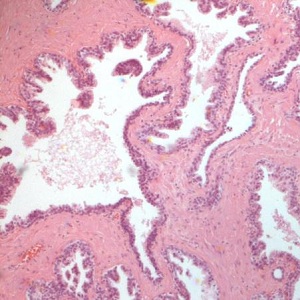
Biopsy of the prostate, stained by Haematoxylin-eosin technique, is the first step for confirming the diagnosis of malignancy. By viewing the microscopic images, pathologists determine the histological grade of the tumor and assess prognosis of the patient. The most widespread method of grading for determining prognosis in the prostate cancer was developed by Gleason during the 1970s [27]. This diagnosis is subjective, fractal analysis may instead permit to perform an objective, quantitative, classification of the tumor.
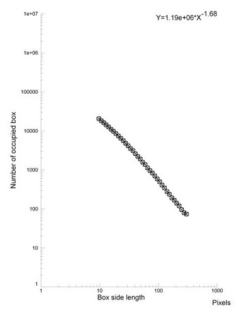
Geometric Complexity (local fractal dimension, D0) may be calculated on the skeletonized images (Figures 2 and 3, bottom, left) by the box-counting methods. Briefly, each skeletonized image is covered by nets of square boxes and the amount of boxes containing any part of the outline is counted. A log-log graph is plotted on the side length of the square against the number of outline-containing squares. If our image is fractal, a linear segment appears: the slope of the linear segment of the graph represents the local fractal dimension of the image (Figures 2 and 3; bottom, right). In our example, a normal prostate tissue and a prostate cancer, the log-log plots used to calculate the local fractal dimension of the images shows one line (from 300 to 10 pixels; 1 pixel = 1 micrometer) with high correlation coefficient, always above a value equal to 0.99, thus justifying our fractal analysis.
In effect, prostate cancer is a recent field where fractal analysis has been applied with remarkable success, showing that fractal dimension is able to correlate to the severity of the injury [28,29].
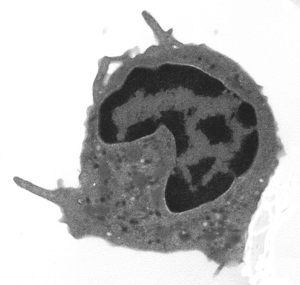
We can also show an example of fractal analysis performed by the evaluation of Entropy, measure of the amount of “disorder” presented in the image, applied on cells in diabetes, an atherosclerosis-linked disease. Monocytes present high geometric complexity of their surface in subjects affected by diabetes mellitus, a severe pathology where one of the major vascular complication is an accelerated atherosclerosis. The high complexity of the monocytic surface is linked to the hyperactivation of these blood cells, one of the cause/complication of the disease. If one observes those cells at high magnification, monocytic surfaces show a fractal structure (its log-log plot is linear, the surface has homothety, see, Figure 4) and fractal analysis may be performed, permitting to distinguish between them.
To evaluate the information (Entropy) presents in the patterns, information dimension, D1, a robust estimate from a finite amount of data that gives the probability of finding a point in the image, is calculated [30]. The skeletonized image is covered with boxes of linear size, d (as above), but now keeping track of the mass, mi (the amount of pixels) in each box, and calculated the information entropy from the summation of the number of points in the i-th box divided by the total number of points in the set multiplied for its logarithm. The slope of the log-log plot of information entropy vs. 1/box side length represented the information dimension of the distribution. The log-log plot used to calculate the information dimensions shows a line from 300 to 10 pixels (0.3 – 0.01 mm) with high correlation coefficient, always above a value equal to 0.99 (Figure 4), thus justifying our fractal approach(both the methodologies, D0 and D1 fractal dimension, are always validated by measuring computer-generated Euclidean and fractal shapes of known fractal dimensions. In our experience inter- and intra-observer error of the entire procedure are < 3%).
Changes in vasculature geometric complexity is another field in which fractal analysis is emerging as a reliable model to quantify and describe morphological aspects of microvessels [33], with potential implications in future clinical and surgical applications, as well as to follow antiangiogenic therapy, in pituitary adenoma, glioblastoma multiforme and other brain malignant tumors [34,35]. In effect, potent mathematical models based on fractal analysis of tumor vasculature are growing in order to perform diagnosis and predict responses to therapies of cancer [33,36].
We show the use of other fractal indexes performed by us in order to study microvessel distribution in Down syndrome and in Ehlers-Danlos syndrome, such as the Lempel-Ziv index, or “randomness”, and the Fractal Dimension of the Minimum Path or “tortuosity”.
To determine the algorithmic complexity or “randomness” of the vascular pattern, the microvessel network image is vectorialized and the relative Lempel-Ziv value is calculated [37,38]. More precisely, vascular network lattices from a 251 x 251 pixels window of the original image is transformed into 16,732 points containing one dimensional vector, where each datum point has been converted into a single binary digit according to whether the skeletenozide image of the microvessel network is touched ( =1) or not ( = 0). Relative LZ values are close to 0 for a deterministic equation and close to 1 for a totally destructured random phenomenon.
Dmin is computed for each vascular cluster from the power law (lc = r Dmin), where Dmin is the exponent that governs the dependence of the minimum path length between two points (lc) on the Pythagorean distance (r) between them in a fractal random material. The slope of the log-log plot represented Dmin [39]. In our approach, the half perimeter and the maximum diameter of either the vessel loops or vessel free areas is measured using an automated procedure and Dmin is calculated: for each sample 500-1,000 areas are measured, the slope of the log-log plot represents Dmin [38].
In Down syndrome as well in Ehlers-Danlos syndrome, Dmin and LZ values of the microvessel networks of the vestibular oral mucosa are changed in comparison with healthy subjects permitting to discover a unknown characteristic of the subject (a higher “density” of the microvessel network, presumably linked to his/her hypermobility, [38,40,41] (Figure 5)).
Since one hundred year the pathologist examines under a microscope the histopathological images of bioptic samples removed from patients, and makes judgments based on their personal experience. Pathologists typically assess the change in the distribution of the cells across the tissue under examination and the deviations in the cell structures themselves. However, this judgment is subjective, and often leads to considerable variability, sometimes with low levels of concordance among the pathologists. To improve the reliability of diagnosis, it is important to develop computational tools for quantitative diagnosis that operate on quantitative measures. Such computerized diagnosis facilitates objective mathematical judgment complementary to that of a pathologist, providing objective “numbers”. Today, following Mandelbrot’s work, nonlinear, fractal, approaches grow in importance. Fractality, the geometric concept related to highly irregular shapes, that originates from simple iterated function with non-integer, or fractional, dimensions, and a property known as self-similarity, give to the pathologist a powerful method to support diagnosis and prognosis of the patients.
In the present day, evidence-based medicine (EBM) is the fundamental element to evaluate the effects of drugs, surgery or other interventions, on health outcomes. EBM requires randomized controlled trials and well tested analytical techniques. So, even if there is undoubted support for the effectiveness of the fractal approaches in human pathology to support differential diagnosis and prognosis, limitations of the major part of the extant research concerning fractal analysis are present: a few double-blind tests for quantifying sensitivity and specificity of the fractal approaches and the need to compare these nonlinear techniques with an appropriate gold standard technique. A receiver-operator characteristic (ROC) analysis, Bayesan analysis, k-NN, and vector machine classifiers, are necessary in order to evaluate the sensitivity and specificity of these techniques in pathology [28,42,43]. Nonetheless, it is certains that the use of fractal analysis in human pathology be a field with a very promising future.

![]()

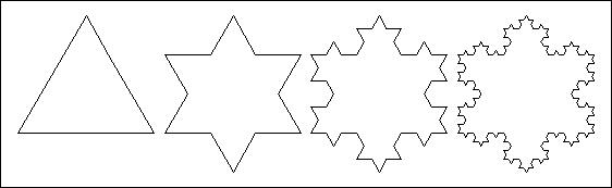 |
| Figure 1: Koch snowflake, a theoretical fractal that begins with an equilateral triangle and then replaces the middle third of every line segment with a pair of line segments (endlessly) |
 |
|
 |
 |
| Figure 2: Hematoxylin-Eosin stained prostate specimen in a healthy subject (top); its contours obtained after segmentation (bottom, left); its log-log plot obtained by fractal analysis (bottom, right). Note that in the fantastic complexity of the biological feature is possible to recognize a log-log linear scaling (p<0.01) that permits an objective characterization of the image (the fractal dimension, corresponding to the exponent of the log-log straight line) | |
 |
|
 |
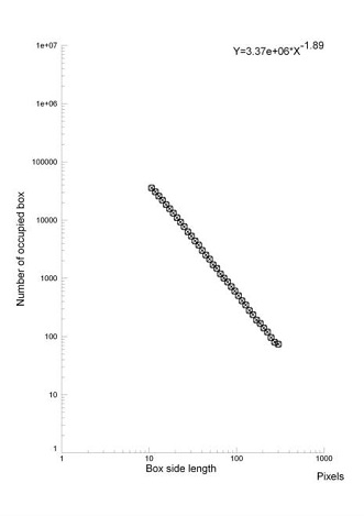 |
| Figure 3: Hematoxylin-eosin stained prostate cancer (top); its contours obtained after segmentation (bottom, left); its log-log plot obtained by fractal analysis (bottom, right).Note that the picture appears even more complex than in healthy (see Figure 2). Also here, it is possible to recognize a log-log linear scaling (p<0.01) but the fractal dimension, the exponent of the log-log straight line, is higher than in healthy (see, Figure.2). Original magnification, x 40 ROC curves reveal the powerful discrimination ability among healthy tissue and prostatic cancer by fractal analysis (Table.1) | |
 |
 |
 |
 |
| Figure 4: A monocyte (transmission electron microscopy, x 3700) in a healthy subject (top) and in a type 2 diabetes mellitus (below). The exponent of the straight line is the entropy of the monocytic surface, measure of the amount of disorder presented in the image: fractal analysis distinguishes between the monocyte at rest of healthy subjects and the activated monocyte of type 2 diabetes mellitus [31,32] | |
 |
| Figure 5: Microvessel network of the vestibular oral mucosa and its skeletonized binary image (top). In Down syndrome and in Ehlers-Danlos syndromes the tortuosity index is decreased and randomness index (LZ) is increased (bottom) [38,40,41], meaning an increase of randomness |
Samples |
Sensitivity |
Specificity |
D0, CUT-OFF |
AUC |
P |
|---|---|---|---|---|---|
Normal vs cancer (Gleason 6-9) |
0.98 |
0.96 |
1.73 |
0.992 |
0.0001 |
Normal vs Gl. 6 |
0.93 |
0.96 |
1.73 |
0.97 |
0.0001 |
Normal vs Gl. 8 |
1.00 |
0.96 |
1.73 |
0.999 |
0.0001 |
Table 1: High discriminating power of fractal dimension index (D0), normal tissue vs. cancer, every Gleason indexes or low and high Gleason indexes |
|||||