Open Access
Research Article
Max Screen >>
ISSN: 2455-765X
Copyright: © 2018 Frempong NK. This is an open-access article distributed under the terms of the Creative Commons Attribution License, which permits unrestricted use, distribution, and reproduction in any medium, provided the original author and source are credited.
Related article at Pubmed, Google Scholar
In this paper, the objective was to study differential factors that explains the mortality rates of male pensioners, comparing the survival patterns of early and normal retirees through a non-parametric approach and a Cox-Proportional Hazard model .The data used was obtained from the Social Security and National Insurance Trust (SSNIT)-Ghana which spans from 1st January, 1990 through 14th June, 2014. The time to death after retirement was the main outcome considered as a counting process.
At the end of the study, overall survival experience through non-parametric methods such as Kaplan-Meier and Nelson-Aalen estimators was estimated. The Kaplan-Meier survival estimation shows significant differences in survival pattern between normal retirees and early retirees. Overall, 50% of the male pensioners is expected to have died, approximately by age 77 years. Generally, retirees with lower employment duration have relatively high hazards of death after retirement and those in the high income group stays much longer.
Results from the Cox-PH model showed that, male pensioners who joined the pension scheme at older ages have more risk of death after retirement, pensioners who earned high total income have lower risk of death after retirement and male pensioners who have worked more years have high risk of death after retirement. Male pensioners who retire normal with high total income have more chance of death after retirement as compared to pensioners who retire early with high total income and vice-versa.
Keywords: Pensioners; Heterogeneity; Cox Proportional Hazard; Kaplan-Meier; Mortality
In many areas of mortality investigations the main goal or objective is to model the mortality data in order to explain mortality rates or hazards and forecast. However, sometimes the interest goes behind this objective and the aim is to study differential factors or heterogeneity that explains the mortality rates. This last situation corresponds to studies where the particular type of designs implies to gather the data in groups or clusters. A social security pension plan specifically a defined benefit plan, where the amount a pensioner is paid is based on how many years employed and the salary one have earned. The design of such plan follows a longitudinal study where members join the scheme at entry age and contribute monthly until date of retirement. The contribution in some percentage of the monthly income which the employer pays on your behalf. In the very last years there has been a growing interest in modelling different levels of mortality pattern for pensioners.
There have been several studies which detected no survival differences between those who take early retirement and normal retirees [1]. There is an underlying assumption which states that, the survival patterns of early retirees and normal retirees are homogeneous but in reality, the survival patterns could differ. Retirees seek to maximize their well-being not at a single point in time but over time. A retiree with long employment duration and high retirement income transfers consumption into the retired years which in effect is determined by the quantum of his/her pension income [2], In history, a retiree is bound to face mortality once he/she joins the scheme. Pension schemes face large and unpredictable risks when retirees tend to live longer than expected which may affect the sustainability of the funds. To address this problem, the employment duration and total income (amount paid as gratuity) are taken into account in modeling the mortality of the male retirees whilst adjusting for entry age as an onset of risk.
The main objective of this paper is to study differential factors that explain the mortality of the pensioners, to compare the survival and hazards of these differential factors through the use of non-parametric and to semi-parametric methods.
Several models consider the concepts of this mixture of laws: models of frailty [3], combined fragility), common shocks models, Cox regression model Cox, (1972), Nelson-Aalen (additive hazard) decomposition Aalen, (1978), combinations of both, etc., [4,5]. In actuarial models concept, the Cox model and more recently, the Aalen’s models, are widely used, especially in reference to their ease of implementation and interpretation, and also as a result of the occurrence of censoring (right) and left truncation are been considered.
The hazard function is given as:
Time to death after retirement is a time to event data and an example of a stochastic process. The male pensioners data may be described as a counting process which is a random function of time, denoted as N(t) . When t=0 , the count is zero and constant over time except that, at each point in time when an event occurs, it jumps. A counting process, N(t) expressed as
The probability space defined as (F,P,Ω), such that Ω is the sample space, F is the σ - field and is the measure of probability defined on F .
A random phenomenon that is time dependent is known as a stochastic process denoted as

A stochastic process X is customized to history of information (filtration) Ft if for every t≥0, X(t) is measurable and hence,
In many statistical applications in the context of stochastic process, martingales play an important role. It is observed that expressing functions (true parameter estimates evaluated) and the distinction between estimators and actual values observed are martingales.
In relation to filtration, Ft , a martingale is a stochastic system M that satisfies the following conditions:
(i) M is adopted to Ft.
E\M(t)\< for all t .
with the martingale property
Consider T* and C , two independent random variables and non-negative. The time to the occurrence of a particular event is denoted by the random variable T* . It can be time to death after retirement. As in the case of this study, it is time to death of male pensioners after retirement. In several studies, the exact time T* may additionally by no means be known because it is able to be censored at time C , this is, one simplest observes the minimum value of
where the intensity process λ(t) is regarded a predicted process. The counting process N(t) is then said to contain intensity process λ . When the intensity process is a function of a risk and hazard functions, it turns out that the model part, also known as the compensator is
Kaplan-Meier Estimator: Considering the entire lifetimes of all male pensioners in this study, there are cases when data obtained are incomplete, especially in the form of right censoring cases of survival times after retirement. It results in a case that, one does not fully observe the survival times, the distribution of the survival times as well as the cumulative hazard function can still be estimated. The Nelson-Aalen and Kaplan-Meier estimator in this case of right-censored survival data are described. The Nelson-Aalen estimator is an estimator of the cumulative hazard function [9-11];

The Cox model takes the form;

Cox (1972) proposed this PH model. Estimates of the log-relative risk parameter β are normally derived and shown with the cumulative baseline hazard function
The Cox model takes the form;

The descriptive summaries of the study outcomes "Alive" and "Death" are presented in Table 1 and 2 respectively. A total of 30,268 male pensioners were classified into "Alive" and "Death" status based on the data information. From Table 1, overall there are 14774 male pensioners death and 15494 male pensioners who were alive as at June 2014. Out of the remaining male pensioners who were alive, about 40% retired early (55-59 years) and 60% retired normal or compulsory retirement age (60 years and above). Of the combined data loss of lives, about 70% had retired normal and 30% retired early. For Alive male pensioners, the average employment duration, entry age and total income are 28.1 years, 31 years and GHS 11723.49 respectively. For retirees who have died the average employment duration, entry age and total income are 27.4 years, 34.2 years and GHS 4114.58 respectively. Employees who retired normal had maximum entry age of 46 years to the scheme, maximum total amount of GHS 401649.55 paid. Employees who retired early had the minimum entry age of 19 years with minimum employment duration of 12 years. The two sample t-test using Satterthwaite approximation of unequal variances showed highly significant difference (t=-15.06, p<0.0001) in employment duration between the two groups of retirement. Similarly, there was a highly significant difference in entry age (t=-67.82, p<0.0001) and total income (t=-6.82, p<0.0001) amongst the two groups of retirees. Conditioning on status of an alive male pensioner, there is significant differences in employment duration, entry age and total income (t=-11.59, p<0.0001; t=-48.82, p<0.0001; t=-17.47, p<0.0001) . Similarly, on status of death, highly significant differences in employment duration, entry age and total income (t=-13.17, p<0.0001; t=-43.61, p<0.0001; t=-5.80, p<0.0001) were observed. Correlation analysis was performed within the two groups of retirees and the overall data. Spearman correlation test was considered because of the non-normal nature of the data. For early retirement, the failure time (time to death after retirement) is significantly correlated with employment duration (ρ=-0.134, p<0.0001) , entry age (ρ=0.102, p<0.0001) and total income (ρ=0.324, p<0.0001).
For normal retirement, the failure time is significantly correlated with employment duration (ρ=-0.0709, p<0.0001) and total income (ρ=0.381, p<0.0001) but not significant with entry age (ρ=0.122, p<0.111). For the combined data, the failure time is significantly correlated with all the three factors ( = -0.106,p<0.0001;ρ=-0.025,p<0.0001;ρ<0.349,ρ<0.0001). Some of the observed correlations are weak even though they are significant. The direction and size of the correlation coefficient show consistent results of significant linear relationship between time to death and employment duration, time to death and total income. Even though the time to death is weakly related to employment duration and almost stronger with total income. Time to death and entry age showed inconsistent results.
The results indicate that male pensioners with longer employment duration have shorter survival periods and vice versa.
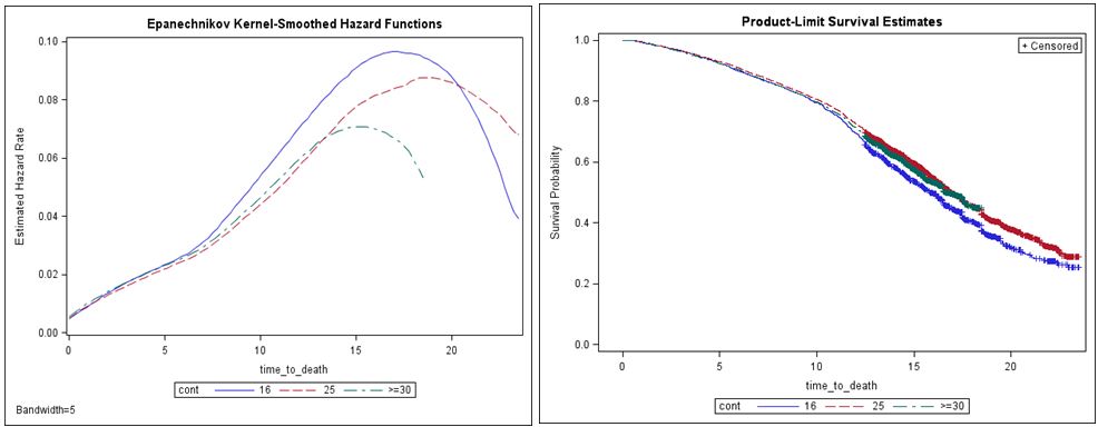
In this section the overall survival experience through a non-parametric methods, such as Kaplan-Meier and Nelson-Aalen estimators were considered. These methods were employed to estimate the survival and cumulative hazards. The overall median survival time is about 21 years 6 months after retirement. Thus beyond 21 years 6 months, 50% of the male pensioners is expected to have died at an approximate age of 77 years. The overall survival is stratified by retirement group, censored observations are represented by vertical ticks on the graph (Figure 1) below. Because the observation with the longest survival time is censored, the survival function will not decay to zero (0). Instead, the survival function will remain at the survival probability estimated at the previous interval.
Kaplan–Meier (KM) survival of early retirees is greater than the normal retirees at all time intervals. The log rank test shows a highly significant results (log rank test= 704.03, df=1, p < 0.0001). It appears that employees who retire normal generally have a worse survival experience. Standard nonparametric techniques do not typically estimate the hazard function directly. So we explored the hazard rate using a graph of the kernel-smoothed estimate. We generally expect the hazard rate to change smoothly over time. To accomplish this smoothing, the hazard function estimate at any time interval is a weighted average of differences within a window of time that includes many differences, known as the bandwidth. The time to death are further stratified by the levels of employment duration. The smoothed lines in Figure 2(a) are labeled by the midpoint of employment duration in each group. From the plot we can see that the hazard of death after retirement appears lower at the lower ages of retirement and then increases monotonically until a time that it shows some concavity. The hazard function is also generally lower for the two highest employment duration categories after 12 years of retirement. We observe varying peaks of hazards for each employment duration category. The green and brown curves representing the two highest employment duration categories is truncated on the right because the last persons in those groups died long before the end of the study. Figure 2(b) shows the survival curves of each employment duration category. We observe that survival until 11 to 12 years after retirement looks similar for each category. However the significant difference (logrank test=24.33, df=3, p<0.0001) shows after 13 years of retirement from age 55 years. Thus significant survival risk is after age 68 years for male pensioners based on employment duration categories.
Early retirees with lower employment duration have relatively high hazards of death as in Figure 3a. However, normal retirees with lower employment duration have relatively high hazards and a continuosly increasing hazards over time, as shown in Figure 3b. This may be due to lager number at risk at longer periods. There is a significant differences in the survival patterns of the level of employment duration within the group of retirement.
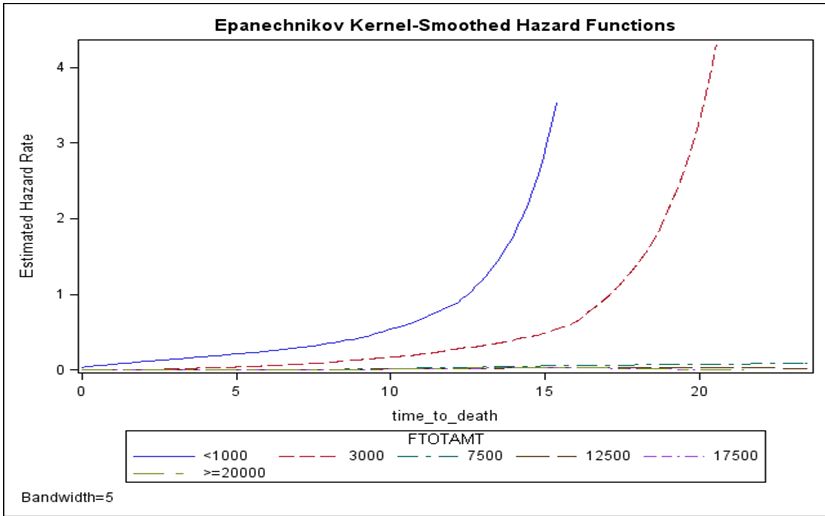
From the Figure 4, we observe that the hazard function appears lower at the beginning of retirement time for all total income categories and then increases exponentially for lower income groups. The hazard function stays low and mostly constant for higher income groups. Pensioners in the higher income category stays much longer as expected.
Finally, the cumulative hazard function is estimated using the Nelson-Aalen estimator. The cumulative hazard shows the expected number of deaths at each observed retirement time. The Nelson-Aalen estimate of 15 years after retirement for the overall, normal, early data samples are 0.539, 0.665 and 0.343 respectively. The interpretation of the overall estimate is that we expect 0.539 deaths (per person) by the end of 15 years after retirement. The early retirement group shows the least cumulative hazard compared to normal retirement group. This exploratory analysis informed us what the requirements of the model are to allow for multiple risk factors simultaneously and allow risk factors to vary their impact by age.
In this section, estimates of the standard Cox proportional hazard models are presented. Four models (M1, M2, M3 and M4) were considered and all models were fitted. In Table 2, the estimated models with model fit statistics with a suitable model selected are shown.
From Table 2, it was observed that four models M1, M2, M3 and M4 were estimated. The AICs for models M1, M2, M3 and M4 are 261485.24, 260075.79, 255400.17 and 255398.21 respectively. Model M1 was estimated with 4 parameters, model M2 with 5 parameters, model M3 with 6 parameters and model M4 was estimated with 9 parameters.
Focusing on the regression result as shown in Table 3 below, the estimated parameter, standard errors of the parameters and a test are presented. All the main and interaction effects are highly significant.
The parameters with positive effect on the hazards are Entry age (onset of risk), retire, (Total income * retire), (Employment duration * Employment duration), (Total income * Total income) and those with negative effect on the hazards are Employment duration, Total income, (Entry age * retire), (Employment duration * retire).
Before applying the Cox model the continuous covariates were therefore centered around their average value to obtain a hazard function for an individual with average covariate values (for the continuous variates).
Due to the principle of parsimony, model M3 is chosen to be the suitable model even though the AIC for model M4 is smaller than M3.From Table 4, the results of the MLE shows model coefficients, tests of significance and hazard ratios. For every year increase in entry age, the hazard increases about 1%, which means that, pensioners who joined the scheme at older ages have more risk of death after retirement. Adjusting for entry age, retirement status have no effect on mortality when all other factors remain unchanged.
For a unit increase in total income, the hazard decreases by 1% indicating that, a male pensioner with high total income has low risk of death than a male pensioner with low total income. An increase in the employment duration increases the hazard to about 9%. This indicates that, male pensioners who have more contribution periods have high risk of death compared to male pensioners with lower contribution periods.The effect of an interaction retire *total income is significant whilst the effect of interaction retire*employment duration is not significant. The interaction effect of retire *employment duration has no effect on mortality. For the significant interaction effect of retire *total income, male pensioners who retire normal with high total income have more chance of death as compared to male pensioners who retire early with high total income. Male pensioners who retire normal with low total income also have more chance of death compared to male pensioners who retire early with low total income.
From the findings of the Kaplan-Meier estimation, there is significant differences in survival pattern between normal retirement and early retirees. Overall, 50% of the male pensioners are expected to have died, approximately by 77 years. The results of Nelson-Aalen estimation shows early retirees with lower employment duration have relatively high hazards of death after retirement and normal retirees with lower employment duration have relatively high hazards of death after retirement. Pensioners in the high income group stays much longer than pensioners in the low income group. From the findings of the Cox-PH model, the significant differential factors that have effect on mortality are entry age, employment duration and total income whilst retirement status have no effect on mortality. It is therefore concluded from the Cox-PH model that, male pensioners who joined the pension scheme at older ages have more risk of death after retirement, pensioners who earned high total income have lower risk of death after retirement and male pensioners who have worked more years have high risk of death after retirement. Male pensioners who retire normal with high total income have more chance of death after retirement as compared to pensioners who retire early with high total income and vice-versa.

![]()

 |
| Figure 1: Kaplan-Meier survival curves since retirements |
.JPG) |
| Figure 2(a): Estimated hazards by employ dur (b) KM survival by employ dur |
.JPG) |
| Figure 2(b): Estimated hazards by employ dur (b) KM survival by employ dur |
 |
| Figure 3 a: Estimated hazards for early retirement data by employ dur (b) Estimated hazards for normal retirement data by employ dur |
 |
| Figure 4: Estimated hazard of overall data by level of total income |
Status |
||||||||
|---|---|---|---|---|---|---|---|---|
Alive |
n |
Summary Statistics |
Emp. Dur. (yrs) |
Entry age (yrs) |
Total income (GHS) |
|||
Combined |
15494 |
Mean |
28.1 |
31.0 |
11723.49 |
|||
Std. Deviation |
4.9 |
5.5 |
9022.22 |
|||||
Median |
29.0 |
30.0 |
9222.49 |
|||||
Mode |
30.0 |
30.0 |
7021.44 |
|||||
Minimum |
15.0 |
19.0 |
4820.49 |
|||||
Maximum |
35.0 |
46.0 |
401649.55 |
|||||
Early Retirement |
6215 |
Mean |
27.9 |
28.6 |
10292.64 |
|||
Std. Deviation |
4.8 |
4.9 |
6964.68 |
|||||
Median |
28.0 |
28.0 |
8469.76 |
|||||
Mode |
29.0 |
26.0 |
7021.14 |
|||||
Minimum |
15.0 |
19.0 |
4941.19 |
|||||
Maximum |
35.0 |
43.0 |
270279.15 |
|||||
Normal Retirement |
9279 |
Mean |
28.5 |
32.6 |
2681.86 |
|||
Std. Deviation |
4.9 |
5.3 |
10057.34 |
|||||
Median |
30.0 |
32.0 |
9855.55 |
|||||
Mode |
34.0 |
30.0 |
9109.75 |
|||||
Minimum |
15.0 |
24.0 |
4820.49 |
|||||
Maximum |
35.0 |
46.0 |
401649.55 |
|||||
Death |
n |
Summary Statistics |
Emp. Dur. (yrs.) |
Entry age (yrs.) |
Total income (GHS) |
|||
Combined |
14774 |
Mean |
27.0 |
33.0 |
3972.89 |
|||
Std. Deviation |
5.0 |
5.6 |
4891.96 |
|||||
Median |
28.0 |
32.0 |
2635.91 |
|||||
Mode |
30.0 |
30.0 |
1115.89 |
|||||
Minimum |
12.0 |
19.0 |
208.1 |
|||||
Maximum |
35.0 |
46.0 |
153899.18 |
|||||
Early Retirement |
4405 |
Mean |
26.2 |
30.20 |
3639.36 |
|||
Std. Deviation |
4.9 |
4.9 |
4292.99 |
|||||
Median |
27.0 |
29.0 |
2809.62 |
|||||
Mode |
29.0 |
26.0 |
1115.89 |
|||||
Minimum |
12.0 |
19.0 |
308.4 |
|||||
Maximum |
35.0 |
44.0 |
153899.18 |
|||||
| Normal Retirement | 10369 |
Mean |
27.4 |
34.2 |
4114.58 |
|||
Std. Deviation |
5.1 |
5.5 |
5118.90 |
|||||
Median |
28.0 |
34.0 |
2571.44 |
|||||
Mode |
30.0 |
30.0 |
1326.28 |
|||||
Minimum |
14.0 |
24.0 |
208.1 |
|||||
Maximum |
35.0 |
46.0 |
87635.22 |
|||||
Table 1: Summary statistics of the “Alive” and “Death” variables |
||||||||
Model |
Parameters |
AIC |
|||
M1 |
4 |
261485.24 |
|||
M2 |
5 |
260075.79 |
|||
M3 |
6 |
255400.17 |
|||
M4 |
9 |
255398.21 |
|||
Table 2: The estimated models with model fit statistics |
|||||
Parameter |
Estimate |
Standard Error |
|||
Main Effects |
|||||
|---|---|---|---|---|---|
Entry age |
0.1102** |
0.01198 |
|||
Employment duration |
-0.382** |
0.01995 |
|||
Total income |
-5.9x10⁻⁴** |
-5.99x10⁻⁶** |
|||
Retire |
6.774** |
0.7109 |
|||
Interaction Effects |
|||||
Entry age*retire |
-0.11188** |
0.01252 |
|||
Emp. duration*retire |
-0.12666** |
0.01274 |
|||
Total income*retire |
0.0001189** |
6.354x10⁻⁶ |
|||
Emp. duration*Emp. duration |
0.0115** |
0.000316 |
|||
Total income* Total income |
1.1569x10⁻⁹** |
1.099x10⁻¹¹ |
|||
Table 3: Parameter estimates and standard errors of M4 |
|||||
Parameter |
DF |
Par. Estimate |
SE |
Chi-Square |
Pr>Chi-Sq |
Hazard Ratio |
|||
Entry age |
1 |
0.00768 |
0.00337 |
5.1984 |
0.0226 |
1.008 |
|||
Total Income |
1 |
-0.00055 |
|
8899.6232 |
<0.0001 |
0.999 |
|||
Emp. duration |
1 |
0.08915 |
0.00497 |
321.7393 |
<0.0001 |
1.093 |
|||
Retire |
1 |
-0.00416 |
0.11540 |
0.0013 |
0.9712 |
0.996 |
|||
Ret * total income |
1 |
0.00916 |
|
423.1368 |
<0.0001 |
1.009 |
|||
ret * emp. duration |
|
0.0007143 |
0.00433 |
0.0272 |
0.8690 |
1.001 |
|||
Table 4: Maximum Likelihood Estimates of Model M3 |
|||||||||